利用朴素贝叶斯算法进行文档分类
在 scikit-learn 里,朴素贝叶斯算法在 sklearn.naive_bayes 包里实现,包含了本章介绍的几种典型的概率分布算法。其中 GaussianNB 实现了高斯分布的朴素贝叶斯算法,MultinomialNB 实现了多项式分布的朴素贝叶斯算法,BernoulliNB 实现了伯努利分布的朴素贝叶斯算法。本文我们用 MultinomialNB 来实现文档自动分类。如果你不熟悉朴素贝叶斯算法,可参阅笔者的另外一篇博客零基础学习朴素贝叶斯算法。
1 获取数据集
本节使用的数据集来自 mlcomp.org 上的 20news-18828,免费注册后即可下载。下载完数据集后,可以解压解压到 ~/code/datasets/mlcomp/ 目录下,解压后会在 ~/code/datasets/mlcomp 下生成一个名为 379 的目录,其目录下包含三个子目录和一个名为 metadata 的介绍文件:
$ cd ~/code/datasets/mlcomp
$ ls 379
metadata  raw  test  train
我们将使用 train 子目录下的文档进行模型训练,然后使用 test 子目录下的文档进行模型测试。train 子目录下包含 20 个子目录,每个子目录代表一种文档的类型,子目录下的所有文档都是属于目录名称所标识的文档类型。读者朋友可以随意浏览数据集,以便对数据集有一个感性的认识。比如 datasets/mlcomp/379/train/rec.autos/6652-103421 ,这是一个纯广本文件,可以使用任何文本编辑器打开。这是一个讨论汽车主题的帖子:
Hahahahahaha. gasp pant Hm, I’m not sure whether the above was just a silly remark or a serious remark. But in case there are some misconceptions, I think Henry Robertson hasn’t updated his data file on Korea since…mid 1970s. Owning a car in Korea is no longer a luxury. Most middle class people in Korea can afford a car and do have at least one car. The problem in Korea, especially in Seoul, is that there are just so many privately-owned cars, as well as taxis and buses, the rush-hour has become a 24 hour phenomenon and that there is no place to park. Last time I heard, back in January, the Kim Administration wanted to legislate a law requireing a potential car owner to provide his or her own parking area, just like they do in Japan.
Also, Henry would be glad to know that Hyundai isn’t the only car manufacturer in Korea. Daewoo has always manufactured cars and I believe Kia is back in business as well. Imported cars, such as Mercury Sable are becoming quite popular as well, though they are still quite expensive.
Finally, please ignore Henry’s posting about Korean politics and bureaucracy. He’s quite uninformed.
2 文档的数学表达
怎么样把一个文档表达为计算机可以理解并处理的信息?这是自然语言处理里的一个重要课题,完整的内容可以写成鸿篇巨著。本节简单介绍 TF-IDF 的原理,以便读者更好地理解本文介绍的实例。
TF-IDF 是一种统计方法,用以评估一个词语对于一份文档的重要程度。TF 表示词频 (Term Frequency),对一份文档而言,词频为特定词语在这篇文档里出现的次数除以文档的词语总数。比如一篇文档总共有 1000 个词,其中 “朴素贝叶斯” 出现了 5 次,“的” 出现了 25 次,“应用” 出现了 12 次,那么它们的词频分别是 0.005, 0.025, 0.012。
IDF 表示一个词的逆向文档频率指数 (Inverse Document Frequency) ,可以由总文档数目除以包含该词语的文档的数目,再将得到的商取对数得到,它表达的是词语的权重指数。比如,我们的数据集总共有 10000 篇文档,其中 “朴素贝叶斯” 只出现在 10 篇文档中,则其权重指数 $IDF = log(\frac {10000} {10}) = 3$ 。“的” 在所有的文档中都出现,则其权重指数 $IDF = log(1) = 0$ 。“应用” 在 1000 篇文档中出现,则其权重指数 $IDF = log(\frac {10000} {1000}) = 1$ 。
计算出每个词的词频和权重指数后,两者相乘,即可得到这个词在文档中的重要程度。词语的重要性随着它在文档中出现的次数成正比增加,但同时会随着它在语料库中出现的频率成反比下降。关于 TF-IDF 在搜索引擎上的应用,可参阅吴军老师的《数学之美》里的《如何确定网页和查询的相关性》一文。
有了 TF-IDF 这个工具,我们就可以把一篇文档转换为一个向量。首先,可以从我们的数据集(在自然语言处理领域,也称为 corpus ,即语料库)里提取出所有出现的词语,我们称为词典。假设词典里总共有 10000 个词语,则每个文档都可转化为一个 10000 维的向量。其次,针对我们要转换的文档里出现的每个词语,都去计算其 TF-IDF 的值,并把这个值填入文档向量里,这个词所对应的元素上。这样就完成了把一篇文档转换为一个向量的过程。一个文档往往只会由词典里的一小部分词语构成,这就意味着这个这个向量里大部分元素都是零。
所幸,上述过程我们不需要自己写代码完成,scikit-learn 软件包里实现了把文档转换为向量的过程。首先,我们把训练用的语料库读入内存:
from time import time
from sklearn.datasets import load_files

print("loading train dataset ...")
t = time()
news_train = load_files('datasets/mlcomp/379/train')
print("summary: {0} documents in {1} categories.".format(
    len(news_train.data), len(news_train.target_names)))
print("done in {0} seconds".format(time() - t))
我们的代码保存在 ~/code/ 目录下,其相对路径 datasets/mlcomp/379/train 目录下放的就是我们的语料库,其中包含 20 个子目录,每个子目录的名字表示的是文档的类别,子目录下包含这种类别的所有文档。load_files() 函数会从这个目录里把所有的文档都读入内存,并且自动根据所在的子目录名称打上标签。其中,news_train.data 是一个数组,里面包含了所有文档的文本信息。news_train.target 也是一个数组,包含了所有文档所属的类别,而 news_train.target_names 则是的类别的名称,因此,如果我们想知道第一篇文档所属的类别名称,只需要通过代码 news_train.target_names[news_train.target[0]] 即可得到。
上述代码在笔者电脑上的输出是:
loading train dataset ...
summary: 13180 documents in 20 categories.
done in 0.212177991867 seconds
不难看到,我们的语料库里,总共有 13180 个文档,其中分成 20 个类别。接着,我们需要把这些文档全部转换为由 TF-IDF 表达的权重信息构成的向量:
from sklearn.feature_extraction.text import TfidfVectorizer

print("vectorizing train dataset ...")
t = time()
vectorizer = TfidfVectorizer(encoding='latin-1')
X_train = vectorizer.fit_transform((d for d in news_train.data))
print("n_samples: %d, n_features: %d" % X_train.shape)
print("number of non-zero features in sample [{0}]: {1}".format(
    news_train.filenames[0], X_train[0].getnnz()))
print("done in {0} seconds".format(time() - t))
其中,TfidfVectorizer 类是用来把所有的文档转换为矩阵,该矩阵每行都代表一个文档,一行中的每个元素代表一个对应的词语的重要性,词语的重要性由 TF-IDF 来表示。熟悉 scikit-learn API 的读者应该清楚,其 fit_transform() 方法是 fit() 和 transform() 合并起来。其中,fit() 会先完成语料库分析,提取词典等操作,transform() 会把对每篇文档转换为向量,最终构成一个矩阵,保存在 X_train 变量里。这段代码在笔者电脑上的输出为:
vectorizing train dataset ...
n_samples: 13180, n_features: 130274
number of non-zero features in sample
  [datasets/mlcomp/379/train/talk.politics.misc/17860-178992]: 108
done in 4.15024495125 seconds
由程序的输出,我们可以知道,我们的词典总共有 130274 个词语,即每篇文档都可转换为一个 130274 维的向量(这是一个巨大的向量)。第一篇文档中,只有 108 个非零元素,即这篇文章由 108 个单词组成,其单词数大于等于 108 个(因为有些词可出现多次)。在这篇文档中出现的这 108 个单词的 TF-IDF 值会被计算出来,并保存在向量中的指定位置上。X_train 是一个维度为 13180 x 130274 的稀疏矩阵(这是一个巨稀疏的矩阵)。
3 模型训练
费了好些功夫,终于把文档数据转换为 scikit-learn 里典型的训练数据集矩阵:矩阵的每一行表示一个数据样本,矩阵的每一列表示一个特征。接着,我们可以直接使用 MultinomialNB 来对数据集进行训练:
from sklearn.naive_bayes import MultinomialNB

print("traning models ...".format(time() - t))
t = time()
y_train = news_train.target
clf = MultinomialNB(alpha=0.0001)
clf.fit(X_train, y_train)
train_score = clf.score(X_train, y_train)
print("train score: {0}".format(train_score))
print("done in {0} seconds".format(time() - t))
其中 alpha 表示平滑参数,其值越小,越容易造成过拟合,值太大,容易造成欠拟合。这段代码在笔者电脑上的输出为:
traning models ...
train score: 0.997875569044
done in 0.274363040924 seconds
接着,我们加载测试数据集,并拿一篇文档来预测看看是否准确。测试数据集在 ~/code/datasets/mlcomp/379/test 目录下,我们用上文介绍的相同的方法,先加载数据集:
print("loading test dataset ...")
t = time()
news_test = load_files('datasets/mlcomp/379/test')
print("summary: {0} documents in {1} categories.".format(
    len(news_test.data), len(news_test.target_names)))
print("done in {0} seconds".format(time() - t))
在笔者的电脑上的输出为:
loading test dataset ...
summary: 5648 documents in 20 categories.
done in 0.117918014526 seconds
可见,我们的测试数据集总共有 5648 篇文档。接着,我们把文档向量化:
print("vectorizing test dataset ...")
t = time()
X_test = vectorizer.transform((d for d in news_test.data))
y_test = news_test.target
print("n_samples: %d, n_features: %d" % X_test.shape)
print("number of non-zero features in sample [{0}]: {1}".format(
    news_test.filenames[0], X_test[0].getnnz()))
print("done in %fs" % (time() - t))
这里需要注意,vectorizer 变量是我们处理训练数据集时用到的广本向量化的类 TfidfVectorizer 的实例,此处我们只需要调用 transform() 进行 TF-IDF 数值计算即可,不需要再调用 fit() 进行语料库分析了。这段代码在笔者电脑上的输出为:
vectorizing test dataset ...
n_samples: 5648, n_features: 130274
number of non-zero features in sample
    [datasets/mlcomp/379/test/rec.autos/7429-103268]: 61
done in 2.915759s
这样,我们的测试数据集也转换为一个维度为 5648 x 130274 的稀疏矩阵。我们可以取测试数据集里第一篇文档初步验证一下,看看我们训练出来的模型能否正确地预测这个文档所属的类别:
pred = clf.predict(X_test[0])
print("predict: {0} is in category {1}".format(
    news_test.filenames[0], news_test.target_names[pred[0]]))
print("actually: {0} is in category {1}".format(
    news_test.filenames[0], news_test.target_names[news_test.target[0]]))
这段代码在笔者电脑上的输出为:
predict: datasets/mlcomp/379/test/rec.autos/7429-103268 is in category rec.autos
actually: datasets/mlcomp/379/test/rec.autos/7429-103268 is in category rec.autos
看来预测的和实际的是相符的。
4 模型评价
显然,我们不能通过一个样本的预测来评价模型的准确性。我们需要对模型有个全方位的评价,所幸 scikit-learn 软件包提供了全方位的模型评价工具。
首先,我们需要对测试数据集进行预测:
print("predicting test dataset ...")
t0 = time()
pred = clf.predict(X_test)
print("done in %fs" % (time() - t0))
在笔者的电脑上输出:
predicting test dataset ...
done in 0.090978s
接着,我们使用 classification_report() 函数来查看一下针对每个类别的预测准确性:
from sklearn.metrics import classification_report

print("classification report on test set for classifier:")
print(clf)
print(classification_report(y_test, pred,
                            target_names=news_test.target_names))
在笔者电脑上的输出为:
classification report on test set for classifier:
MultinomialNB(alpha=0.0001, class_prior=None, fit_prior=True)
                          precision    recall  f1-score   support

             alt.atheism       0.90      0.91      0.91       245
           comp.graphics       0.80      0.90      0.85       298
 comp.os.ms-windows.misc       0.82      0.79      0.80       292
comp.sys.ibm.pc.hardware       0.81      0.80      0.81       301
   comp.sys.mac.hardware       0.90      0.91      0.91       256
          comp.windows.x       0.88      0.88      0.88       297
            misc.forsale       0.87      0.81      0.84       290
               rec.autos       0.92      0.93      0.92       324
         rec.motorcycles       0.96      0.96      0.96       294
      rec.sport.baseball       0.97      0.94      0.96       315
        rec.sport.hockey       0.96      0.99      0.98       302
               sci.crypt       0.95      0.96      0.95       297
         sci.electronics       0.91      0.85      0.88       313
                 sci.med       0.96      0.96      0.96       277
               sci.space       0.94      0.97      0.96       305
  soc.religion.christian       0.93      0.96      0.94       293
      talk.politics.guns       0.91      0.96      0.93       246
   talk.politics.mideast       0.96      0.98      0.97       296
      talk.politics.misc       0.90      0.90      0.90       236
      talk.religion.misc       0.89      0.78      0.83       171

             avg / total       0.91      0.91      0.91      5648
从输出可以看出来,针对每种类别,都统计了查准率,召回率和 F1-Score。对这些概念不熟悉的读者可参阅笔者的另外一篇博客机器学习系统的设计与调优。此外,我们还可以通过 confusion_matrix() 函数,来生成混淆矩阵,观察每种类别被错误分类的情况,比如,这些被错误分类的文档是被错误分类到哪些类别里的:
from sklearn.metrics import confusion_matrix

cm = confusion_matrix(y_test, pred)
print("confusion matrix:")
print(cm)
在笔者电脑上的输出为:
confusion matrix:
[[224   0   0   0   0   0   0   0   0   0   0   0   0   0   2   5   0   0   1  13]
 [  1 267   5   5   2   8   1   1   0   0   0   2   3   2   1   0   0   0   0   0]
 [  1  13 230  24   4  10   5   0   0   0   0   1   2   1   0   0   0   0   1   0]
 [  0   9  21 242   7   2  10   1   0   0   1   1   7   0   0   0   0   0   0   0]
 [  0   1   5   5 233   2   2   2   1   0   0   3   1   0   1   0   0   0   0   0]
 [  0  20   6   3   1 260   0   0   0   2   0   1   0   0   2   0   2   0   0   0]
 [  0   2   5  12   3   1 235  10   2   3   1   0   7   0   2   0   2   1   4   0]
 [  0   1   0   0   1   0   8 300   4   1   0   0   1   2   3   0   2   0   1   0]
 [  0   1   0   0   0   2   2   3 283   0   0   0   1   0   0   0   0   0   1   1]
 [  0   1   1   0   1   2   1   2   0 297   8   1   0   1   0   0   0   0   0   0]
 [  0   0   0   0   0   0   0   0   2   2 298   0   0   0   0   0   0   0   0   0]
 [  0   1   2   0   0   1   1   0   0   0   0 284   2   1   0   0   2   1   2   0]
 [  0  11   3   5   4   2   4   5   1   1   0   4 266   1   4   0   1   0   1   0]
 [  1   1   0   1   0   2   1   0   0   0   0   0   1 266   2   1   0   0   1   0]
 [  0   3   0   0   1   1   0   0   0   0   0   1   0   1 296   0   1   0   1   0]
 [  3   1   0   1   0   0   0   0   0   0   1   0   0   2   1 280   0   1   1   2]
 [  1   0   2   0   0   0   0   0   1   0   0   0   0   0   0   0 236   1   4   1]
 [  1   0   0   0   0   1   0   0   0   0   0   0   0   0   0   3   0 290   1   0]
 [  2   1   0   0   1   1   0   1   0   0   0   0   0   0   0   1  10   7 212   0]
 [ 16   0   0   0   0   0   0   0   0   0   0   0   0   0   0  12   4   1   4 134]]
从第一行数据可以看出来,类别 0 (alt.atheism) 的文档,有 13 个文档被错误地分类到类别 19 (talk.religion.misc) 里。当然,我们还可以把混淆矩阵进行数据可视化处理:
# Show confusion matrix
import matplotlib.pyplot as plt

plt.figure(figsize=(8, 8), dpi=144)
plt.title('Confusion matrix of the classifier')
ax = plt.gca()
ax.spines['right'].set_color('none')
ax.spines['top'].set_color('none')
ax.spines['bottom'].set_color('none')
ax.spines['left'].set_color('none')
ax.xaxis.set_ticks_position('none')
ax.yaxis.set_ticks_position('none')
ax.set_xticklabels([])
ax.set_yticklabels([])
plt.matshow(cm, fignum=1, cmap='gray')
plt.colorbar()
plt.show()
在笔者电脑上的输出如下图所示:
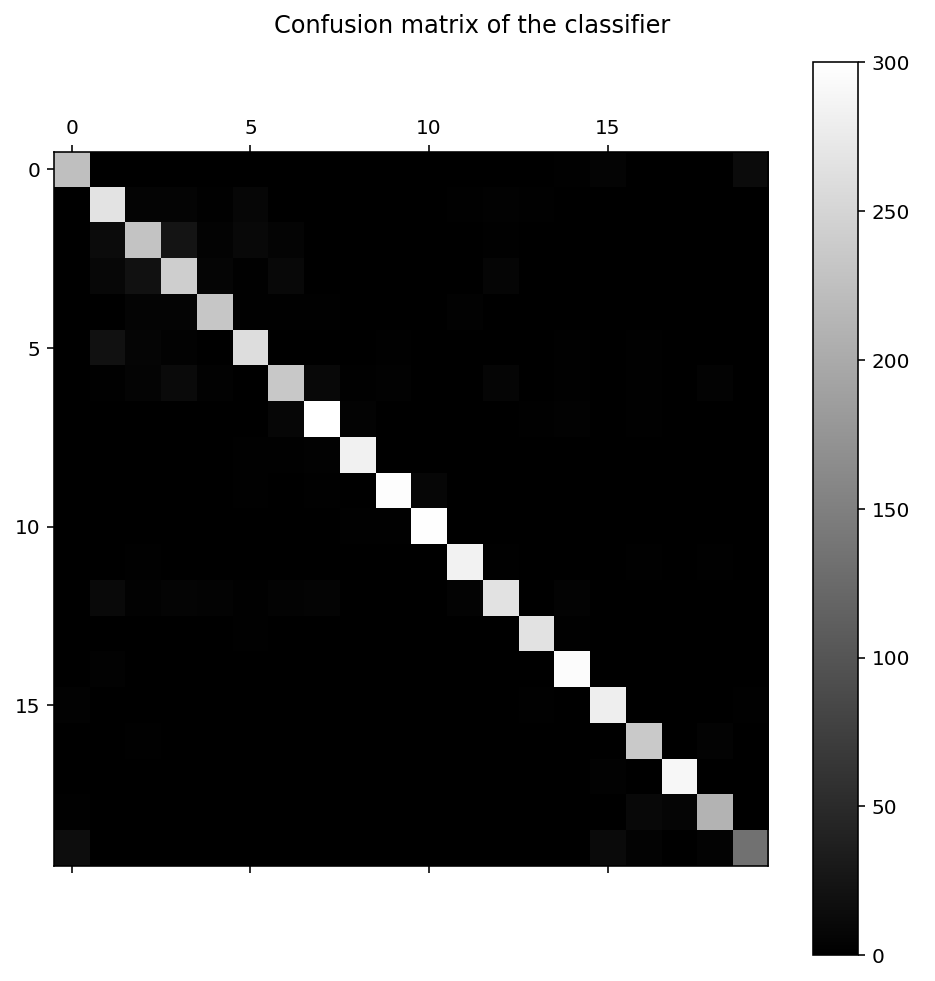
除对角线外,其他地方颜色越浅,说明此处错误越多。通过这些数据,我们可以详细分析样本数据,找出为什么某种类别会被错误地分类到另外一种类别里,从而进一步优化模型。
5 参数选择
MultinomialNB 有一个重要的参数是 alpha ,用来控制模型拟合时的平滑度。我们选择了 0.0001 这个值。实际上,有一个更科学的方法,是利用 scikit-learn 的 sklearn.model_selection.GridSearchCV 来进行自动选择。即我们可以设置一个 alpha 参数的范围,然后让用代码选择出一个在这个范围内最优的参数值。感兴趣的朋友可以阅读 GridSearchCV 的文档偿试一下。
(完)